Logistic and Tent IFS

Recall the tent and logistic maps are among the simplest nonlinear mathematical systems.

Next, recall the coarse-graining method of driving an IFS. The s = 4.0 logistic map has range 0 <= x <= 1, so the four bins are

bin 1	0 <= x < 1/4
bin 2	1/4 <= x < 1/2
bin 3	1/2 <= x < 3/4
bin 4	3/4 <= x <= 1

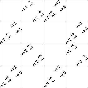
Here is the driven IFS - not random at all, lots of structure. Can we understand its pattern?.

First, we note some address length 2 subsquares appear empty. What are these addresses, and what are the bin-to-bin combinations that cannot occur?

Empty addresses	Forbidden combinations
12	2 -> 1
13	3 -> 1
22	2 -> 2
23	3 -> 2
32	2 -> 3
33	3 -> 3
41	1 -> 4
44	4 -> 4

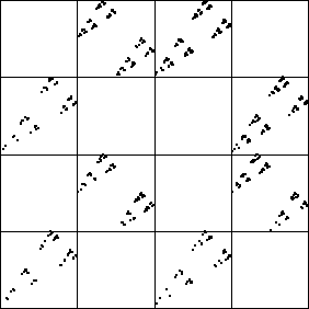
Now suppose we drive the IFS randomly, except that none of the forbidden combinations is allowed. What do we get?

This looks like the original picture. In fact, it is. Another way to see this is to apply the deterministic IFS rules, but imposing the forbidden combinations. Even though this logistic map is chaotic, at least in terms of the driven IFS, it is very simple. Imposing eight forbidden combinations completely determines the driven IFS. In a moment we shall see what characteristic of the s = 4.0 logistic map gives this property.

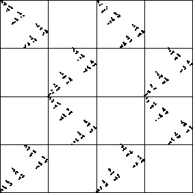
First, here is the driven IFS for the s = 2.0 tent map.

The empty addresses are 12, 13, 22, 23, 31, 34, 41, and 44. And again, imposing the corresponding restrictions generates the same picture. So this, too, is a simple chaotic process.

For another example, consider the s = 3.732 logistic map. We must be a bit careful with the bins in this case.

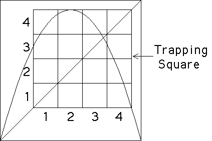
Note the trapping square: graphical iteration shows that points iterate into this square and subsequently never leave. That is, the eventual dynamics are constrained to lie in the trapping square. So we divide the trapping square into bins. What combinations are forbidden? We cannot go

from bin1 into bin1

from bin1 into bin2

from bin2 into bin1

from bin2 into bin2

from bin2 into bin3

from bin3 into bin1

from bin3 into bin2

from bin4 into bin4

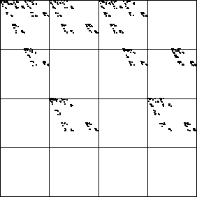
Recall, this is the graph of the function, not the driven IFS. So to find the forbidden combinations, we look above each bin on the bottom of the trapping square and note which bins on the side of the trapping square contain some part of the graph of the function. The left picture is the IFS driven by the s = 3.723 logistic map; the right picture is generated by a random IFS with these restrictions imposed. These ar not the same, so this logistic map is more complex than the s = 4.0 map. Recall every empty subsquare of the right picture has address contaning one of the pairs 11, 12, 13, 21, 22, 23, 32, or 44. Consequently, the left picture has some empty subsquares that are not consequences of the empty pairs. In this sense, the left picture is more complex than the right.

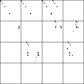
In examples such as the s = 4.0 logistic map, the driven IFS is completely determined by the forbidden pairs. This is because partitioning the range [0, 1] into four equal intervals is a Markov partition.

Finally, suppose we consider systems more complicated than a single logistic map. For example, take N logistic maps and couple each to its nearest neighbors. Letting x¹_t, ..., x^N_t stand for populations 1, ..., N in generation t, we obtain the populations in generation t+1 by

x1t+1 = (1-c)L(x1t) + (c/2)(L(xNt) + L(x2t))

x2t+1 = (1-c)L(x2t) + (c/2)(L(x1t) + L(x3t))

xt+13 = (1-c)L(xt3) + (c/2)(L(xt2) + L(xt4))

...

xN-1t+1 = (1-c)L(xN-1t) + (c/2)(L(xN-2t) + L(xNt))

xNt+1 = (1-c)L(xNt) + (c/2)(L(xN-1t) + L(x1t))

Graphically, we have

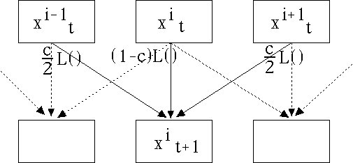
Here c is the coupling constant, a measure how how strongly each value depends on its neighbors. For examaple, c = 0 gives N independent logistic maps: each depends only on itself.

In each generation we measure the average of the xⁱ_t; that is, we measure

zt = (x1t + ... + xNt)/N

What happens if we drive an IFS with z₁, z₂, z₃, ... ?

Let's start with a simple example: N = 2 and s₁ = s₂ = 4. Here the coupling formula becomes

x1t+1 = (1-c)L(x1t) + cL(x2t)

x2t+1 = (1-c)L(x2t) + cL(x1t)

Here we step through the driven IFS for c = 0 to c = 1 in steps of c = 0.1. Many of the pictures look very similar to the driven IFS for a single logistic map. To check this, Here we plot the return maps. Amazingly, we see for some range of coupling values c, the logistic maps synchronize. Note each is chaotic, exhibiting sensitivity to initial conditions, and we did not start them at the same x-value. Nevertheless, they synchronize. Later, we shall see this has applications in secure communication.

Here are some pictures, taking N = 3, s₁ = s₃ = 4.0 and s₂ = 3.2. Do some of these look familiar?

Return to Data-Driven IFS