6. Suppose we know the following time series comes from the logistic map:
0.429, 0.960, 0.150, 0.500, 0.980, 0.077, 0.278, 0.787, 0.657, 0.883, 0.405, 0.945, 0.204, 0.637, 0.906, 0.333, 0.871, 0.440, 0.966.
Without doing a delay plot, can you find the parameter value of the logistic map from the data? Do this by a calculation using two successive values of the time series. Can you see a way to find the parameter value using only one (particular) value of the time series? Answer
7. Suppose we know the following time series
0.859, 0.268, 0.510, 0.932, 0.130, 0.247, 0.470, 0.893, 0.204, 0.388, 0.737, 0.500, 0.950, 0.095, 0.181, 0.344, 0.654, 0.658, 0.649,
comes from either the tent map or from the logistic map. Use a delay plot (by hand) to determine from which it comes. Answer
8. A short time series has the following values: 3.1, 7.9, 8.2, 6.3, 2.8, 4.5. Make a first delay plot of the data. Be sure to label the axes.
9. For the pair of logistic maps
xn+1 = s*xn*(1 - xn)
yn+1 = s*yn*(1 - yn)
suppose x0 and y0 are the same. Suppose an = (xn + yn)/2, the average value of the xn and yn. How will the delay plot of an+1 versus an look? Answer
10.[N] Like the logistic map, the Henon map
xn+1 = yn + 1 - a*xn2
yn+1 = b*xn
exhibits a complicated sequence of bifurcations, but, in fact, the Henon bifurcations are even richer than those of the logistic map. As a very tiny piece of the bifurcation structure, use a calculator to check what happens to the time series starting with (0,0) for the Hnon parameters a = 1.05, b = 0.3. As a and b change, the Henon Map exhibits both periodic and fractal attractors.
In the text, the delay plots we used had a "delay of 1" - that is, from the time series x1, x2, x3, ... we plotted points (x1, x2), (x2, x3), ... . There is no reason to limit ourselves to this scheme. For example, we could use a "delay of 2:" plot points (x1, x3), (x2, x4), ..., or even higher delays. Exercises 11 and 12 investigate some higher delays.
11. Suppose the signal x1, ..., x20 is a real 2-cycle: x1 = x3, x2 = x4,..., x18 = x20, with x1 = 1 and x2 = 2.
(a) Draw the delay plot with a delay of 1 (that is, plot the points (x1, x2), (x2, x3), ..., (x19, x20)). Answer
(b) Draw the delay plot with a delay of 2 (that is, plot the points (x1, x3), (x2, x4), ..., (x18, x20)). Answer
(c) Draw the delay plot with a delay of 3. Answer
(d) Do you see a general pattern emerging? Answer
12. Suppose the signal x1, ..., x20 is a real 3-cycle: x1 = x4, x2 = x5, x33 = x6, ..., x17 = x20, with x1 = 1, x2 = 2, and x3 = 3.
(a) Draw the delay plot with a delay of 1. Answer
(b) Draw the delay plot with a delay of 2. Answer
(c) Draw the delay plot with a delay of 3. Answer
(d) Do you see a general pattern emerging? Answer
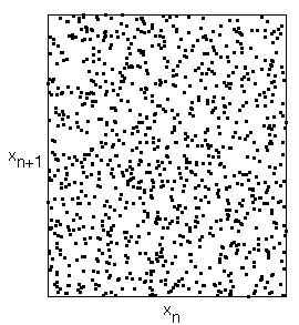
13. Explain why Figure 6.14 looks the way it does. That is, suppose the signal is uniform random, with all x's in the interval [0,1]. Why does the delay plot fill in the unit square uniformly darkly? (Hint: divide the unit square into four subsquares:
S1 = {(xn,xn+1): 0<=xn<1/2, 0<=xn+1<1/2},
S2 = {(xn,xn+1): 1/2<=xn<1, 0<=xn+1<1/2},
S3 = {(xn,xn+1): 0<=xn<1/2, 1/2<=xn+1<1}, and
S4 = {(xn,xn+1): 1/2<=xn<1, 1/2<=xn+1<1}.
Since the xn are uniformly distributed in the interval [0,1], it is equally likely that any xn will be less than 1/2 or greater than 1/2. From this, deduce that any point (xn, xn+1) is equally likely to lie in any of the four squares S1, S2, S3, or S4. Now repeat the argument with the unit square divided into sixteen subsquares S1 = {(xn,xn+1): 0<=xn<1/4, 0<=xn+1<1/4}, ..., S16 = {(xn,xn+1): 15/16<=xn<=1, 15/16<=xn+1<=1}. Can you see how to continue and how this argument gives the desired result?)
Return to Chapter 6 Exercises
Return to Chapter 6 Exercises: The Spectra of Noise
Go to Chapter6 exercises: Close Pairs
Return to Chaos Under Control